From Render Pipeline to GPGPU

When we use the render pipeline for general-purpose computing instead of rendering computations, it means that we are using the GPU for purposes other than drawing pixels. In WebGL, when we treat a Texture as a multi-dimensional array, we can read and compute these arrays through calculations in shaders and output the results. The above sentences briefly summarize the fundamental usage of GPGPU.

Here are a few key concepts:

• Treating Texture as a multi-dimensional array
• Reading and computing the multi-dimensional array through shaders
• Outputting the computed results

Treating Texture as a Multi-Dimensional Array for Calculation and Output

A Texture generally contains four channels, which we can regard as a matrix of size ddc. In each channel, we can store different data, enabling us to load the data we need to accelerate into the GPU by loading the Texture.

const resolution = {
    x : 4,
    y : 4
}
// Load data, assuming the data is single-channel
gl.texImage2D(gl.TEXTURE_2D, 0, gl.LUMINANCE, 
    resolution.x, 
    resolution.y, 
    0, gl.LUMINANCE, gl.UNSIGNED_BYTE, 
    new Uint8Array([
        1, 2, 3, 4,
        5, 6, 7, 8,
        9, 10, 11, 12,
        13, 14, 15, 16
]));

Reading the Multi-Dimensional Array through Shaders

When inputting, if we ensure the Texture size is rectangular, we can correctly read the Texture in the fragment shader using the texture2D function.

We can simulate a $[-1,1]$ clipping space with vertices and create a quadrilateral with vertices from -1 to +1 using two triangles.

gl.bufferData(gl.ARRAY_BUFFER, new Float32Array([
  -1, -1,
   1, -1,
  -1,  1,
  -1,  1,
   1, -1,
   1,  1,
]), gl.STATIC_DRAW);

Then, there are two ways to obtain this data in the fragment shader:

1. Use gl_FragCoord to get the pixel coordinate and then convert it to UV coordinates:

   uniform vec2 u_resolution;     // Assuming we passed in the size of the Texture
   uniform sampler2D textureData; // Texture used to read data
   
   void main() {
       vec2 texCoord = gl_FragCoord.xy / resolution;
       // Sample data from the texture
       vec4 data = texture2D(textureData, texCoord);
       // Perform some computation on the data
       vec4 result = someComputation(data);
       // Output the computed result
       gl_FragColor = result;
   }
   

2. Use vertex data transfer in the vertex shader and use interpolation results to obtain UV coordinates:

   vec4 a_position;
   varying vec2 index;
   
   void main() {
       index = (a_position.xy + 1.0) / 2.0; 
       gl_Position = a_position;
   }
   

   Then, in the fragment shader, since the passed data will be automatically interpolated in the fragment, index will be the UV coordinates:

   varying vec2 index;    // Texture coordinates passed from the vertex shader
   uniform sampler2D textureData; // Texture used to read data
   
   void main() {
       vec4 data = texture2D(textureData, index);
       // Perform some computation on the data
       vec4 result = someComputation(data);
       // Output the computed result
       gl_FragColor = result;
   }
   

Outputting the Computed Results

You can read the output using gl.readPixels. Note that this output will include all four RGBA channels.

Example: Slime Simulation

Slime Simulation Overview

This simulation is based on a diffusion mechanism model for the slime mold Physarum polycephalum as described in the paper¹. As shown in the image below:

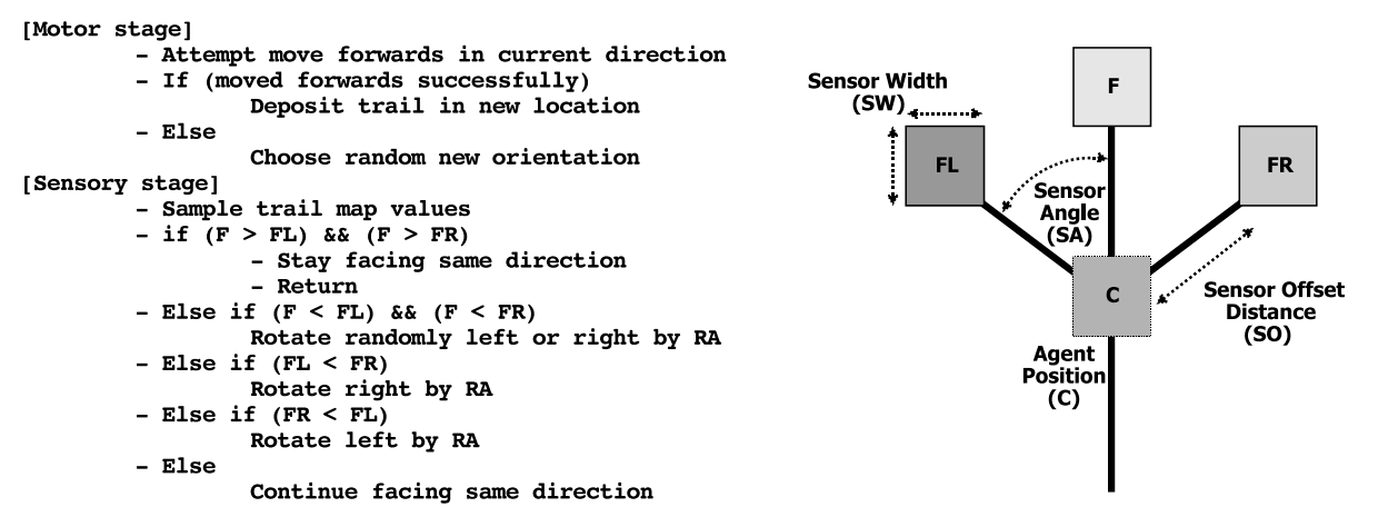
In brief, the slime mold leaves behind pheromones as it moves forward, while simultaneously deploying sensors in the forward direction. The sensors are fixed in three directions, labeled F, FL, and FR in the image. These sensors detect the pheromone trails left by previous movements, leading the mold to prefer moving towards the direction with the highest concentration of pheromones. If the slime mold encounters an obstacle, it will randomly choose a direction to continue moving.

We used WebGL to create the effect of the slime mold's movement and employed GPGPU for accelerated computation, resulting in the effect demonstrated in the simulator.The code translation is based on the simulation effect demonstrated in a video using Unity.²

Tip: Adjust the simulation effects by controlling the hyperparameters. If the page becomes unresponsive, please press the "Stop" button.

Implementation Details

Position and Diffusion Data Recording

We use a texture (pos_tex) to record the current position (2D) and orientation angle (1D) of each slime mold. The texture size is set to 1024x1024 with four channels, where the rg channels record the position data and the b channel records the angle data.

public convertToTextureData(positions: number[], angles: number[]) {
    const data = new Float32Array(1024 * 1024 * 4);
    for (let i = 0; i < angles.length; ++i) {
        const src = i * 2;
        const dst = i * 4;
        data[dst] = positions[src];
        data[dst + 1] = positions[src + 1];
        data[dst + 2] = angles[i];
    }
    return data;
}
public createAgents(positions: number[], angles: number[]) {
    const texture = twgl.createTexture(this.gl, {
        src: this.convertToTextureData(positions, angles),
        width: 1024,
        height: 1024,
        min: this.gl.NEAREST,
        wrap: this.gl.CLAMP_TO_EDGE,
    });
    const framebufferInfo = twgl.createFramebufferInfo(this.gl, [
        { attachment: texture, }
    ], 1024, 1024);
    return {
        texture,
        framebufferInfo,
    };
}

Similarly, we use a texture of the same size (spread_tex) to record the pheromones left by the slime mold in the space, initializing it as an empty texture.

Position Update and Diffusion Simulation

The position update follows the slime mold movement model mentioned above. Three directional sensors are set up, and the information from spread_tex is sampled and compared to determine the final direction of movement.

...
...
float sense(vec2 position,float sensorAngle){
    vec2 sensorDir=vec2(cos(sensorAngle),sin(sensorAngle));
    vec2 sensorCenter=position+sensorDir*sensorOffsetDist;
    vec2 sensorUV=sensorCenter/resolution;
    vec4 s=texture2D(spread_tex,sensorUV,sensorSize);
    return s.r;
}
void main(){
    float vertexId=floor(gl_FragCoord.y*agentsTexResolution.x+gl_FragCoord.x);
    vec2 uv=gl_FragCoord.xy/agentsTexResolution;
    vec4 temp=texture2D(tex_pos,uv);
    vec2 position=temp.rg; // rg --> pos
    float angle=temp.b; // b --> angle
    float width=resolution.x;
    float height=resolution.y;
    float random=hash(vertexId/(agentsTexResolution.x*agentsTexResolution.y)+time);
    // sense environment
    float weightForward=sense(position,angle);
    float weightLeft=sense(position,angle+sensorAngleSpacing);
    float weightRight=sense(position,angle-sensorAngleSpacing);
    
    float randomSteerStrength=random;
    
    if(weightForward>weightLeft&&weightForward>weightRight){
        angle+=0.; //F
    }else if(weightForward<weightLeft&&weightForward<weightRight){
        angle+=(randomSteerStrength-.5)*2.*turnSpeed*deltaTime;
    }else if(weightRight>weightLeft){
        angle-=randomSteerStrength*turnSpeed*deltaTime; //FR
    }else if(weightLeft>weightRight){
        angle+=randomSteerStrength*turnSpeed*deltaTime; //FL
    }

    // move agent
    vec2 direction=vec2(cos(angle),sin(angle));
    vec2 newPos=position+direction*moveSpeed*deltaTime;
    // clamp to boundries and pick random angle if hit boundries  
    ...  
    gl_FragColor=vec4(newPos,angle,0);
}

Meanwhile, the diffusion of pheromones is simulated in spread_tex. The current information strength is sampled and smoothed over a 3x3 area around it, with hyperparameters controlling the diffusion (diffuseSpeed) and evaporation (evaporateSpeed) rates.

void main(){
  vec4 originalValue=texture2D(tex,v_texcoord);
  // Simulate diffuse 
  vec4 sum;
  for(int offsetY=-1;offsetY<=1;++offsetY){
    for(int offsetX=-1;offsetX<=1;++offsetX){
      vec2 sampleOff=vec2(offsetX,offsetY)/resolution;
      sum+=texture2D(tex,v_texcoord+sampleOff);
    }
  }
  vec4 blurResult=sum/9.;
  vec4 diffusedValue=mix(originalValue,blurResult,diffuseSpeed*deltaTime);
  vec4 diffusedAndEvaporatedValue=max(vec4(0),diffusedValue-evaporateSpeed*deltaTime);
  gl_FragColor=vec4(diffusedAndEvaporatedValue.rgb,1);
}

Rendering

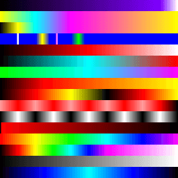
The simulation results are visualized based on the pheromone intensity and the slime mold's position. Sixteen color schemes were generated for the simulation, stored in a texture, and sampled according to position and intensity to achieve the final visualization effect.